Numerical

Q1 - Semi-average (odd)

Solution using the Semi‑Average Method

We have sales data from 2018 to 2023:

1. Split into two equal halves

• First half: 2018–2020

• Second half: 2021–2023

2. Compute the “semi‑averages” (means) for each half

Q1.a) Semi-average - odd

Data

There are 7 years → the middle year is 2018 (Sales = 160). We split the remaining 6 observations into two equal halves:

• First half: 2015, 2016, 2017

• Middle (excluded): 2018

• Second half: 2019, 2020, 2021

1. Compute semi‑averages

Q2.

Q3.

Q4.

Given Data

YT- link Fitting of y=ab^x curve || Curve Fitting || 18mat41 || Dr Prashant Patil

Q5. Pending

Quadratic Trend Analysis: Y = a + bX + cX²

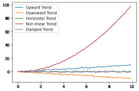
Computing Trend Values Using a Second-Degree (Quadratic) Equation

To compute trend values using a second-degree (quadratic) equation, we need to fit a model of the form: Y=a+bX+cX2

Where:

• Y is the output (dependent variable)

• X is the year (independent variable)

• a,b,c are the coefficients we need to find.

For ease of calculation, we will convert the years into 'time' indices, where the middle year is set to 0.

Given Data:

Step 1: Assign Time Indices (X)

Since there are 5 data points (an odd number), we can assign X=0 to the middle year, 2018.

From the table, we get the following summations:

• n=5 (number of data points)

• ∑Y=1370

• ∑X=0

• ∑X2=10

• ∑X3=0

• ∑X4=34

• ∑XY=285

• ∑X2Y=2765

Step 2: Set up Normal Equations

For a second-degree (quadratic) equation Y=a+bX+cX2, the normal equations are:

1. ∑Y=na+b∑X+c∑X2

2. ∑XY=a∑X+b∑X2+c∑X3

3. ∑X2Y=a∑X2+b∑X3+c∑X4

Substitute the summation values into the normal equations:

4. 1370=5a+b(0)+c(10)⟹1370=5a+10c (Equation A)

5. 285=a(0)+b(10)+c(0)⟹285=10b (Equation B)

6. 2765=a(10)+b(0)+c(34)⟹2765=10a+34c (Equation C)

Step 3: Solve the Normal Equations for a, b, and c

From Equation B: 10b=285 b=10285​ b=28.5

Now we have a system of two equations (A and C) with two unknowns (a and c): A) 5a+10c=1370 C) 10a+34c=2765

Multiply Equation A by 2 to eliminate 'a': 2×(5a+10c)=2×1370 10a+20c=2740 (Equation A')

Subtract Equation A' from Equation C: (10a+34c)−(10a+20c)=2765−2740 14c=25 c=1425​ c≈1.7857

Substitute the value of c back into Equation A to find 'a': 5a+10(1.7857)=1370 5a+17.857=1370 5a=1370−17.857 5a=1352.143 a=51352.143​ a≈270.4286

Step 4: Write the Trend Equation

The quadratic trend equation is: Y=a+bX+cX2 Y=270.4286+28.5X+1.7857X2

Step 5: Compute Trend Values for Each Year

Now, substitute the 'Time (X)' values back into the derived trend equation to find the trend values (Y^).

• For Year 2016 (X = -2): Y^2016​=270.4286+28.5(−2)+1.7857(−2)2 Y^2016​=270.4286−57+1.7857(4) Y^2016​=270.4286−57+7.1428 Y^2016​=220.5714

• For Year 2017 (X = -1): Y^2017​=270.4286+28.5(−1)+1.7857(−1)2 Y^2017​=270.4286−28.5+1.7857(1) Y^2017​=270.4286−28.5+1.7857 Y^2017​=243.7143

• For Year 2018 (X = 0): Y^2018​=270.4286+28.5(0)+1.7857(0)2 Y^2018​=270.4286+0+0 Y^2018​=270.4286

• For Year 2019 (X = 1): Y^2019​=270.4286+28.5(1)+1.7857(1)2 Y^2019​=270.4286+28.5+1.7857 Y^2019​=300.7143

• For Year 2020 (X = 2): Y^2020​=270.4286+28.5(2)+1.7857(2)2 Y^2020​=270.4286+57+1.7857(4) Y^2020​=270.4286+57+7.1428 Y^2020​=334.5714

Summary of Trend Values:

Q.6.

Trend by Semi‑Average Method (5 marks)

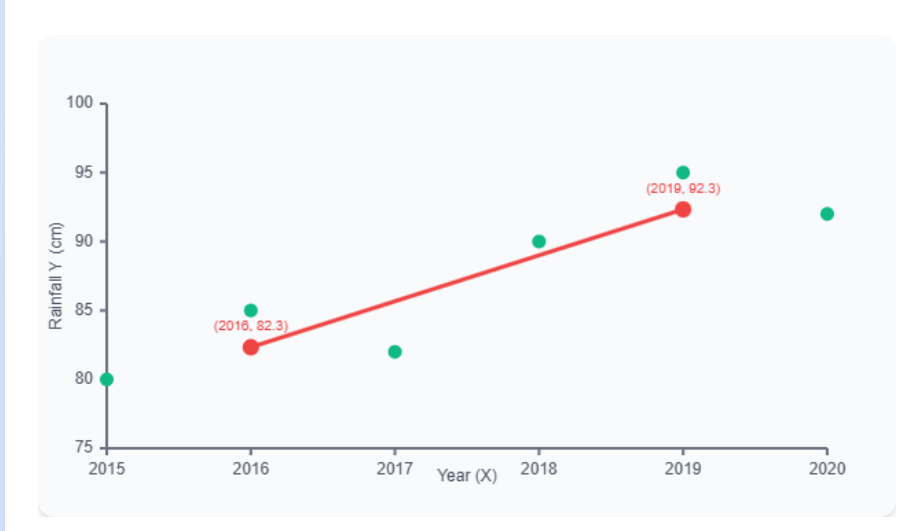
We have annual rainfall YY for Years XX:

1. Split into two equal halves

• First half: 2015–2017

• Second half: 2018–2020

2. Compute semi‑averages

Q7.

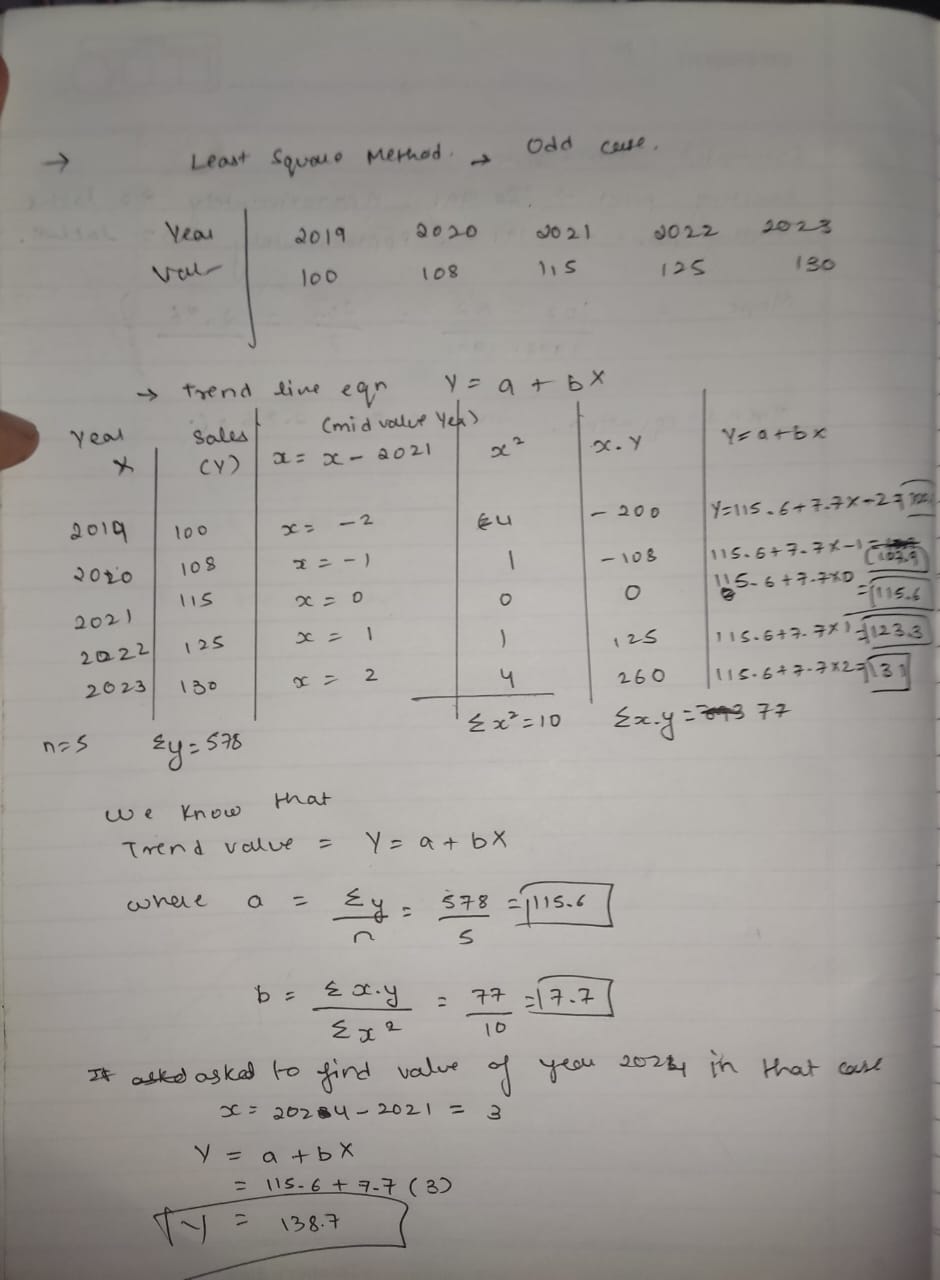
Linear Trend Fitting: Y = a + bX

Given Data

Step 1: Transform Years to Simple Values (X)

Let X = Year - 2018 (using middle year as origin)

Step 2: Set up Normal Equations

For linear trend Y = a + bX, we need:

• ΣY = na + bΣX ...(1)
• ΣXY = aΣX + bΣX² ...(2)

Step 3: Calculate Required Summations

Totals:

• n = 5
• ΣX = 0
• ΣY = 1110
• ΣX² = 10
• ΣXY = 115

Step 4: Form Normal Equations

The normal equations for a linear trend are:

1. ∑Y=na+b∑X

2. ∑XY=a∑X+b∑X2

Substitute the summation values into the normal equations:

1. 1110=5a+b(0)⟹1110=5a (Equation A)

2. 115=a(0)+b(10)⟹115=10b (Equation B)

Substituting the values:

(1) 1110 = 5a + 0b
(2) 115 = 0a + 10b

Step 5: Solve for Coefficients

From equation (1): a = 1110/5 = 222

From equation (2): b = 115/10 = 11.5

Step 6: Linear Trend Equation

Y = 222 + 11.5X

Where X = Year - 2018

Step 7: Calculate Trend Values for Given Years

Step 8: Estimate Value for 2025

For Year 2025: X = 2025 - 2018 = 7

Y₂₀₂₅ = 222 + 11.5(7) = 222 + 80.5 = 302.5

Q8.

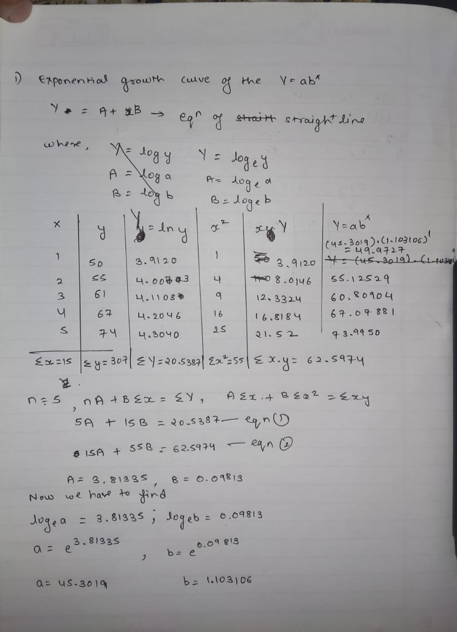
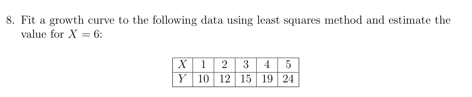
Fitting a Growth Curve using Least Squares Method

Step 1: Create a Calculation Table

We need to compute ln(Y), X2, and Xln(Y) for each data point.

Note: Values for ln(Y) and Xy′ are rounded to 4 decimal places for presentation, but calculations use full precision.

From the table, we have:

• Number of observations, n=5

• ∑X=15

• ∑y′=13.6181

• ∑X2=55

• ∑Xy′=43.0648

Step 2: Set up Normal Equations

The normal equations for the linear form y′=a′+b′X are:

1. ∑y′=na′+b′∑X

2. ∑Xy′=a′∑X+b′∑X2

Substitute the summation values into the normal equations:

1. 13.6181=5a′+15b′ (Equation A)

2. 43.0648=15a′+55b′ (Equation B)

Step 3: Solve for a′ and b′

From Equation A, divide by 5: 2.72362=a′+3b′ ⟹a′=2.72362−3b′

Substitute this expression for a′ into Equation B: 43.0648=15(2.72362−3b′)+55b′ 43.0648=40.8543−45b′+55b′ 43.0648=40.8543+10b′ 10b′=43.0648−40.8543 10b′=2.2105 b′=102.2105​ b′≈0.22105

Now substitute the value of b′ back into the expression for a′: a′=2.72362−3(0.22105) a′=2.72362−0.66315 a′≈2.06047

Step 4: Convert a′ and b′ back to a and b

Remember that a′=ln(a) and b′=ln(b). So, a=ea′ and b=eb′.

a=e2.06047≈7.8505 b=e0.22105≈1.2473

Step 5: Write the Growth Curve Equation

The fitted growth curve equation is: Y=abX Y=7.8505(1.2473)X

Step 6: Estimate the Value for X = 6

Substitute X=6 into the derived growth curve equation: Y6​=7.8505(1.2473)6 Y6​=7.8505×(3.7997) Y6​≈29.829

Conclusion:

The growth curve fitted to the given data using the least squares method is approximately: Y=7.8505(1.2473)X

Using this equation, the estimated value for X=6 is 29.829.

Q9.

Solution (5 marks)

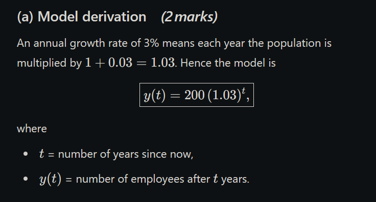
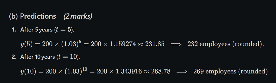
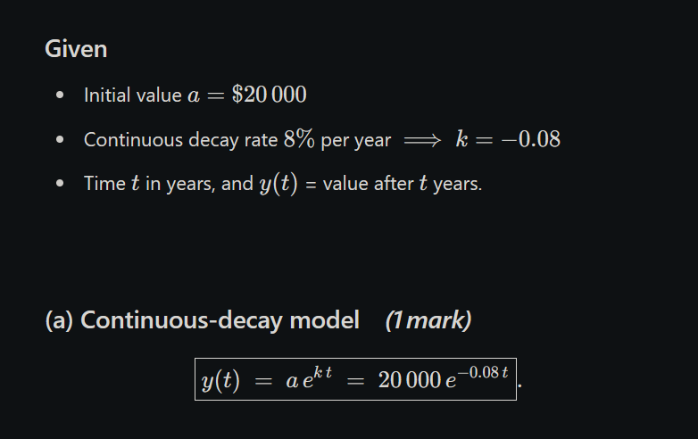
A company starts with y(0)=200y(0)=200 employees and grows at 3% per year. We model this with the discrete‐time exponential growth formula.

(a) Model derivation (2 marks)

(b) Predictions (2 marks)

Answer:

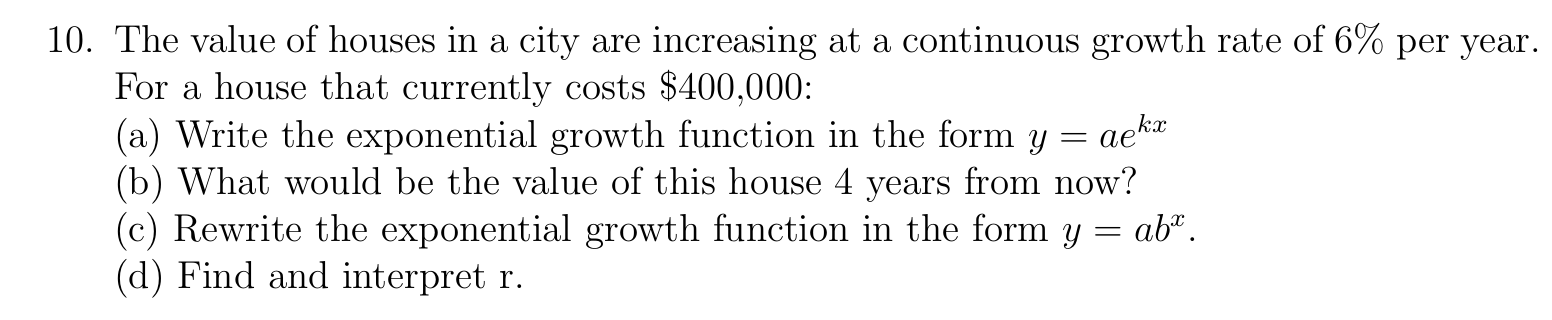
10.

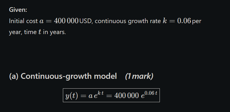
(a) Continuous‐growth model (1 mark)

Substituting Given Values:

• a = $400,000
• k = 0.06
• x = time in years

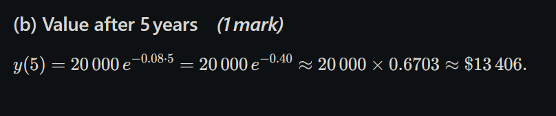
(b) Value after 4 years (1 mark)

Calculate y when x = 4:

y = 400,000e^(0.06 × 4) y = 400,000e^(0.24)

Calculate e^(0.24):

e^(0.24) = 1.271249

House Value After 4 Years:

y = 400,000 × 1.271249 = $508,499.60

(c) Rewrite in the Form y = ab^x (1 mark)

Converting from y = ae^(kx) to y = ab^x:

We need to find b such that: ae^(kx) = ab^x

This means: e^(kx) = b^x

Taking the x-th root of both sides: e^k = b

Calculate b:

b = e^k = e^(0.06) = 1.061837

Exponential Growth Function in y = ab^x form:

y = 400,000(1.061837)^x

Verification:

Let's check if both forms give the same result for x = 4:

• Form 1: y = 400,000e^(0.24) = $508,499.60
• Form 2: y = 400,000(1.061837)^4 = 400,000 × 1.271249 = $508,499.60 ✓

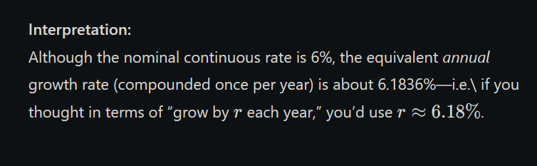
(d) Find and interpret rr (2 marks)

Finding r:

In the form y = ab^x, we have b = 1 + r where r is the effective annual growth rate.

From part (c): b = 1.061837

Therefore: r = b - 1 = 1.061837 - 1 = 0.061837

r = 6.1837% ≈ 6.18%

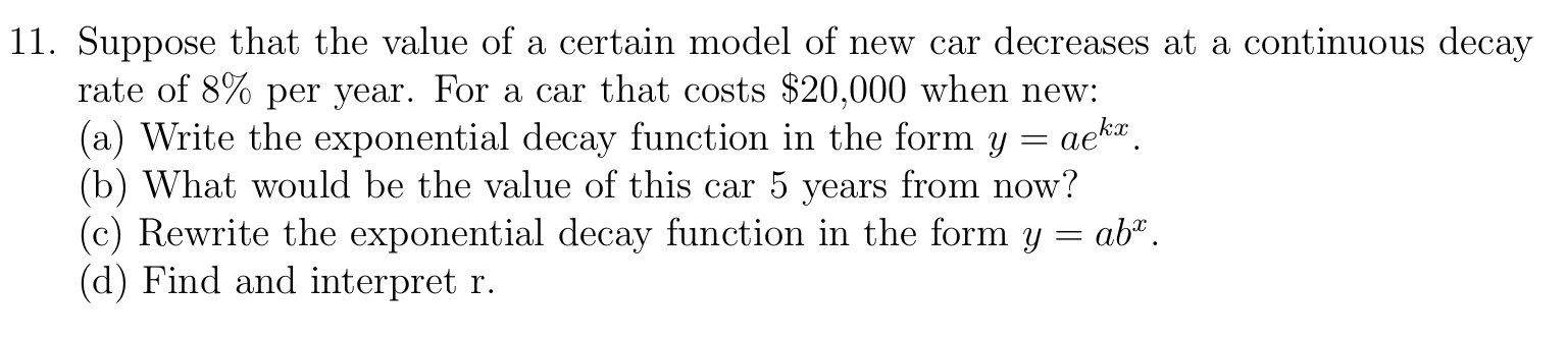
Q11.

y = ae^(kx)

Where:

• y = value after time x
• a = initial value
• e = Euler's number (≈ 2.71828)
• k = continuous decay rate (negative for decay)
• x = time period

(a) Continuous‐decay model (1 mark)

Part (c): Rewrite in the Form y = ab^x

Converting from y = ae^(kx) to y = ab^x:

We need to find b such that: ae^(kx) = ab^x

This means: e^(kx) = b^x

Taking the x-th root of both sides: e^k = b

Calculate b:

b = e^k = e^(-0.08) = 0.923116

Exponential Decay Function in y = ab^x form:

y = 20,000(0.923116)^x

Verification:

Let's check if both forms give the same result for x = 5:

• Form 1: y = 20,000e^(-0.40) = $13,406.40
• Form 2: y = 20,000(0.923116)^5 = 20,000 × 0.670320 = $13,406.40 ✓

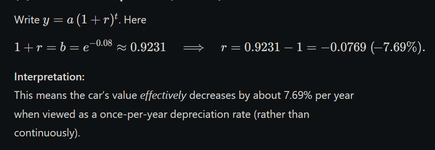
(d) Find and interpret r (2 marks)

Unit 1 : Theory

(6,7,8,9) pending

1. Define time series data. Give two examples from different fields where time series analysis is applied.

Definition:
Time series data is a set of number of observations or values collected over time at regular intervals, like daily, monthly, or yearly or a period of time. The order of time is important when studying this data or performing anlysis.
Characteristics (Simple):
Data is collected over time in order.
The gap between (time interval) each data point is equal (like daily or monthly).
Past Data can affect what Future values.
It shows patterns like increase over time, repeating seasons, or ups and downs.

Examples:
Stock Prices (Finance): It means checking how the price of a company’s share changes every day in the stock market. This helps in understanding trends and making investment decisions.

Weather Data (Meteorology): It means recording the temperature of a place every day. This helps in studying climate patterns and forecasting weather.

OR

Introduction to Time Series

A Time Series is a collection of data points recorded in order over time. These data points are usually taken at regular intervals like daily, monthly, or yearly.
The main goal of time series analysis is to understand patterns (like trends and seasonality) and make future predictions.

Example: Daily temperature, stock prices, or sales of a product over months.

Applications of Time Series in Various Fields
7. Economics & Finance:
- Forecasting stock prices, inflation rates, or exchange rates.

8. Weather Forecasting:

   • Predicting rainfall, temperature, and natural disasters.

9. Healthcare:

   • Monitoring patient health data like heart rate or glucose levels over time.

10. Business & Sales:

    • Predicting future sales, demand, or production planning.

11. Energy Sector:

    • Forecasting electricity consumption and power load management.

Conclusion:
Time Series analysis helps in making data-driven decisions by identifying patterns and predicting future events.

Let me know if you want key terms like trend, seasonality, or forecasting methods explained.

2. What are the main components of a time series? Explain each briefly with an example.

A Time Series is a collection of data points recorded in order over time. These data points are usually taken at regular intervals like daily, monthly, or yearly.
Four Main Components:

1. Trend (T):
Trend shows the long-term direction of the data, either increasing, decreasing, or staying constant over time.
It reflects the overall growth or decline in the data set.

(Slow and steady increase or decrease in data over a long time.)
Example: The population of India has been steadily increasing over the past decades.

2. Seasonal (S):
Seasonal component refers to patterns that repeat at regular intervals, like every month or year. These patterns are influenced by seasons, festivals, or events.

(Patterns that repeat regularly in a fixed time (like every year or month).)
Example: Ice cream sales are always higher during summer months compared to winter.

3. Cyclical (C):
Cyclical patterns are long-term rises and falls in data, but they don’t follow a fixed time period. They are usually related to economic or business cycles.

(Ups and downs in data over a long time but not in a fixed pattern.)

Example: Economic growth and recession cycles that happen roughly every 7 to 10 years.

4. Irregular (I):
Irregular or random components are sudden, unpredictable changes in the data. These are caused by unexpected events like natural disasters or strikes.

(Unexpected or random changes in the data.)
Example: Sudden increase in umbrella sales due to an unexpected heavy rainfall.

3. Explain the purpose of decomposing a time series. How does decomposition help in forecasting?

A Time Series is a collection of data points recorded in order over time. These data points are usually taken at regular intervals like daily, monthly, or yearly.
What is Decomposition?
Decomposition means breaking a complex time series into smaller, simpler parts like trend, seasonal, and irregular components. This helps to clearly see patterns in the data.

Purpose of Decomposition:

• To break down complex data into easy-to-understand parts.
• To find hidden patterns like trends and seasonal changes.
• To remove random, irregular changes and focus on useful patterns.

Benefits for Forecasting:

1. Pattern Recognition: It helps to clearly see trends (increasing/decreasing) and repeating seasonal patterns for future predictions.

2. Model Selection: Once we know the pattern, we can select the best forecasting model to get accurate results.

3. Improved Accuracy: By understanding each part of the data, the predictions become more correct and reliable.

Example: Decomposing retail sales data helps predict holiday season spikes and long-term growth patterns.

Decomposition of Time Series

Definition:
Decomposition means breaking a complex time series into smaller, simpler parts like trend, seasonal,cyclical and irregular components. This helps to clearly see patterns in the data

Main Components of Time Series

1️⃣ Trend (T):
It shows the long-term movement or direction of the data over time.
Slow and steady increase or decrease in data over a long time.
Example: Gradual increase in sales over years.

2️⃣ Seasonal Component (S):
It refers to regular patterns that repeat at fixed periods (like months or quarters).
Patterns that repeat regularly in a fixed time (like every year or month)
Example: Increase in ice-cream sales during summer.

3️⃣ Cyclical Component (C):
It refers to long-term up and down movements not of fixed period, usually related to the business cycle.
Ups and downs in data over a long time but not in a fixed pattern.
Example: Economic booms or recessions.

4️⃣ Irregular/Random Component (I):
It includes Unexpected or random changes in the data
Example: Sudden drop in sales due to natural disaster.

Types of Decomposition Models

12. Additive Model:
    Used when the variation is constant over time.
    Formula:
    Time Series = T + S + C + I

13. Multiplicative Model:
    Used when the variation increases or decreases over time.
    Formula:
    Time Series=T×S×C×I

Importance of Decomposition

• Helps in understanding patterns clearly.
• Useful for forecasting future values.
• Identifies which factor (trend/season/random) affects the data most.

Example:
Sales of umbrellas →
Trend ↑ (overall sales increasing),
Seasonal (high during rainy season),
Random (sudden spikes due to unexpected rain).

Conclusion:
Time series decomposition breaks complex data into simple parts, helping in analysis and forecasting.

4. Describe the free-hand curve method for estimating trend in time series data. What are its advantages and disadvantages?

Definition:
The Free-Hand Curve Method is a simple graphical technique used to estimate the trend in time series data by drawing a smooth curve through the plotted data points by hand.

Steps Involved:

14. Plot the time series data on a graph (Time on X-axis and Values on Y-axis).
15. Draw a smooth curve through the points, balancing the fluctuations above and below the curve.
16. The drawn curve represents the trend of the data.

Advantages:

✅ Simple and Easy to use.
✅ Helps to visually understand the general movement of data.
✅ Useful when the data has irregular fluctuations.

Disadvantages:

❌ Subjective — depends on personal judgment of the person drawing the curve.
❌ Not accurate for forecasting or scientific analysis.
❌ Cannot be used for complex or large datasets.

Conclusion:

The Free-Hand Curve Method is useful for a quick visual estimation of trends but not suitable for accurate or large-scale analysis.

Let me know if you want the steps with an example graph explanation next.

5. What is the method of semi-averages? Explain how it is used to estimate the trend.

Definition:
It is a simple method to estimate the trend in time series by dividing the data into two parts, finding their averages, and then drawing a straight line between them to show the trend.

Example:

Let’s say we have annual sales data (in ₹ lakhs) for 6 years:

Step 1: Divide the data into two equal parts

• First Half (2018–2020): 120, 130, 140

• Second Half (2021–2023): 160, 170, 180

Step 2: Calculate Averages of Each Half

• Average of First Half = (120 + 130 + 140) ÷ 3 = 130

• Average of Second Half = (160 + 170 + 180) ÷ 3 = 170

Step 3: Find Midpoints (Years)

• Midpoint of First Half = 2019

• Midpoint of Second Half = 2022

Step 4: Plot Points and Draw Line

• Now we have two points: (2019, 130) and (2022, 170)

• Draw a straight line between these two points to represent the trend.

Conclusion:

![[SEM 2/Time Series/attachments/Devika's Commerce & Management Academy - 19. Semi Averages - Even Number Method in Time Series form Statistics Subject [VmOZ7_Fjn-s - 885x498 - 8m09s].png]]

6. Explain how to fit an exponential curve Y = abˣ using method of least squares. Derive normal equations.

✅ 1. Form of Curve:

We have to fit the curve: Y = abˣ
Where a and b are constants to be calculated.

✅ 2. Make It Linear (Log Transformation):

Take log on both sides:
log Y = log a + x log b

Let:
Z = log Y, A = log a, B = log b
Now equation becomes:
➡ Z = A + Bx → Looks like a straight-line equation.

✅ 3. Apply Least Squares:

Now use the normal equations for fitting a straight line:

1️⃣ nA + BΣx = ΣZ
2️⃣ AΣx + BΣx² = ΣxZ

Solve these two equations to find A and B.

✅ 4. Find a and b:

• a = antilog(A) = 10^A
• b = antilog(B) = 10^B

➡ Final equation: Y = abˣ

✅ Conclusion:

By converting the exponential to a straight-line form, we can use least squares to calculate a and b, and then get the required exponential curve.

7. Explain how to fit parabolic trend Yt = a + bt + ct² using method of least squares.

✅ 1. Form of the Curve:

We want to fit the curve:
➡ Yt = a + bt + ct²
Where a, b, c are constants to be calculated.

✅ 2. Objective:

We apply Least Squares Method to minimize:
➡ S = Σ(Yi - a - bti - cti²)² → Error should be as small as possible.

✅ 3. Normal Equations:

To solve for a, b, c, we form three normal equations:

1️⃣ n·a + b·Σt + c·Σt² = ΣY
2️⃣ a·Σt + b·Σt² + c·Σt³ = ΣtY
3️⃣ a·Σt² + b·Σt³ + c·Σt⁴ = Σt²Y

Where t = time, Y = actual values.

✅ 4. Simplification (Shortcut):

If we shift the origin to the middle of time → Σt = 0 → Normal equations become easier:

1️⃣ n·a + c·Σt² = ΣY
2️⃣ b·Σt² = ΣtY
3️⃣ a·Σt² + c·Σt⁴ = Σt²Y

Now you can easily solve for a, b, c.

✅ 5. Final Equation:

➡ Y = a + bt + ct² → Gives the parabolic trend of the data.

✅ Conclusion:

This method is used when data shows a curved trend (not straight). Parabolic trends are helpful for capturing increasing or decreasing rates of change over time

8. Explain how to fit power curve Y = aXᵇ using method of least squares.

✅ 1. Form of the Curve:

We have to fit:
➡ Y = aXᵇ
Where a and b are constants to be found.

✅ 2. Make It Linear (Log Transformation):

Take logarithm on both sides to make it linear:
log Y = log a + b log X
Let:
➡ Z = log Y, A = log a, X = log X, B = b
Now the equation is:
➡ Z = A + B·X → Linear form like a straight line.

✅ 3. Apply Least Squares:

Now use normal equations to solve:

1️⃣ nA + BΣX = ΣZ
2️⃣ AΣX + BΣX² = ΣXZ

Solve these equations to find A and B.

✅ 4. Find a and b:

• a = antilog(A) = 10^A

• b = B

➡ Final equation: Y = aXᵇ

✅ 5. Conclusion:

The power curve is used when data grows in a multiplicative way with X raised to some power. It is useful for growth models like area vs. diameter, cost vs. output, etc.

Want a numerical example to practice? Just tell me!

9. Explain how to fit exponential curve Y = aeᵇˣ using method of least squares.

✅ 1. Form of the Curve:

We want to fit the curve:
➡ Y = aeᵇˣ
Where a and b are constants to be calculated.

✅ 2. Make It Linear (Log Transformation):

Take logarithm on both sides:
➡ log Y = log a + bx

Let:
➡ Z = log Y, A = log a, B = b
Now it becomes a straight-line equation:
➡ Z = A + Bx

✅ 3. Apply Least Squares Method:

Use normal equations to find A and B:

1️⃣ nA + BΣx = ΣZ
2️⃣ AΣx + BΣx² = ΣxZ

Solve these equations to get values of A and B.

✅ 4. Find a and b:

• a = antilog(A) = 10^A

• b = B

➡ Final equation becomes: Y = aeᵇˣ

✅ 5. Conclusion:

The exponential curve is useful for growth and decay models, like population growth, radioactive decay, compound interest, etc.

10. Discuss the applications of time series analysis in economics and business.

Time series analysis is widely used in both economics and business for making better decisions, understanding patterns, and forecasting future trends.

A) Applications in Economics

1. Macroeconomic Forecasting:

   • Predicting GDP growth of a country
   • Forecasting inflation rates
   • Analyzing trends in unemployment
   • Studying interest rate changes over time

2. Financial Markets:

   • Predicting stock prices and analyzing market trends
   • Forecasting currency exchange rates
   • Tracking commodity price movements
   • Assessing market risks for better investment decisions

B) Applications in Business

3. Demand Forecasting:

   • Predicting sales for better inventory management
   • Understanding seasonal demand patterns for production planning
   • Estimating market demand for new product launches

4. Operations Management:

   • Optimizing supply chain based on future demand
   • Scheduling production activities efficiently
   • Monitoring product quality over time
   • Tracking cost trends for better budgeting

5. Strategic Planning:

   • Identifying long-term business growth trends
   • Studying market cycles for making investment decisions
   • Monitoring company performance regularly
   • Allocating resources as per future needs

Benefits of Time Series Analysis:

• Helps in data-based decision making

• Reduces risks and uncertainty

• Improves operational efficiency

• Leads to better resource use and cost control

Conclusion:
Time series analysis plays an important role in both economics and business for forecasting, planning, and managing resources effectively.

Let me know if you need it in bullet points only or want it even shorter for quick revision.

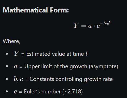
Q11. Gompertz Curve in Time Series

Definition:
The Gompertz Curve is a mathematical model used to fit time series data that shows slow initial growth, followed by rapid growth, and then leveling off.
It is S-shaped (Sigmoid), just like the Logistic Curve, but asymmetrical (not exactly balanced on both sides).

Mathematical Form:

Characteristics of Gompertz Curve:

1️⃣ S-Shaped Growth:

• Starts slowly, grows rapidly, then slows down again.

2️⃣ Asymmetry:

• Growth is not symmetric about the midpoint (unlike the Logistic Curve).

3️⃣ Upper Limit (a):

• The value of aa represents the maximum value that YY approaches but may never fully reach.

4️⃣ Useful for Biological and Market Data:

• Often used to model population growth, spread of diseases, technology adoption, and sales growth.

Merits of Gompertz Curve:

✅ Useful for long-term forecasting of growth data.
✅ Handles cases where growth slows down after a certain point.
✅ Suitable for population studies, economics, marketing, etc.

Demerits of Gompertz Curve:

❌ Complex calculations — requires estimation of multiple constants.
❌ Difficult to fit manually, usually needs statistical software.
❌ Not suitable for data with linear or irregular trends.

Conclusion:

The Gompertz Curve is ideal for predicting growth trends in time series where growth slows over time. However, it requires complex computation and is mainly suitable when S-shaped growth is expected.

Let me know if you want an example solved or graph illustration for better understanding.

UNIT 2:

Time Series Analysis Unit 2 - Exam Answers (7 Marks Each)

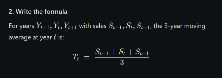
1. Explain the method of moving averages for estimating the trend in a time series. How is it applied?

The moving average method is a mathematical technique used to removes out short-term fluctuations in time series data and finds the approximate long-term trend.
It works by calculating the average of data points over a fixed period.

The Moving Averages Method is a technique used to estimate the trend in a time series by smoothing out short-term fluctuations. It replaces each value in the series with the average of neighboring values.

In simple words:
It gives a smooth line that shows the general direction (trend) of the data over time.

✅ How It Works:

1. Select a time period (like 3, 4, or 5 years) → called the moving average period.

2. Take the average of that many consecutive values.

3. Slide the window forward one time point and repeat the process.

4. The result is a series of moving averages that form the trend line.

✅ Types of Moving Averages:

1️⃣ Simple Moving Average (SMA):
Equal weight to each value.

2️⃣ Centered Moving Average:
Used for even-period averages (like 4-year), where average is centered between years.

✅ Example (3-Year Moving Average):

→ These averages form the trend values.

✅ Advantages:

• Simple and easy to use.

• Smooths out random variations.

• Highlights long-term trend.

❌ Disadvantages:

• Doesn’t work well with seasonal or cyclical data.

• Loses data points at the beginning and end.

• Gives equal weight to all periods (may not reflect reality).

✅ Conclusion:

The Moving Averages Method is a useful technique to smooth time series data and estimate the underlying trend, especially when the data is noisy.

Let me know if you want a diagram or graph to visualize the trend!

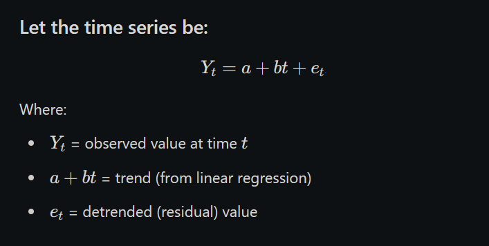
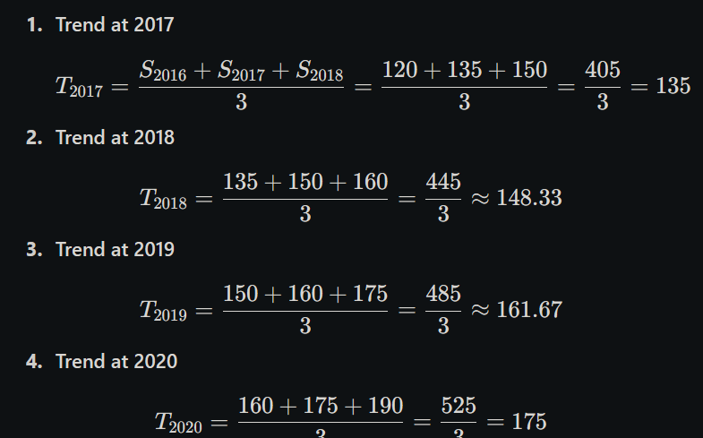
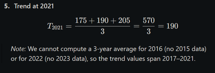
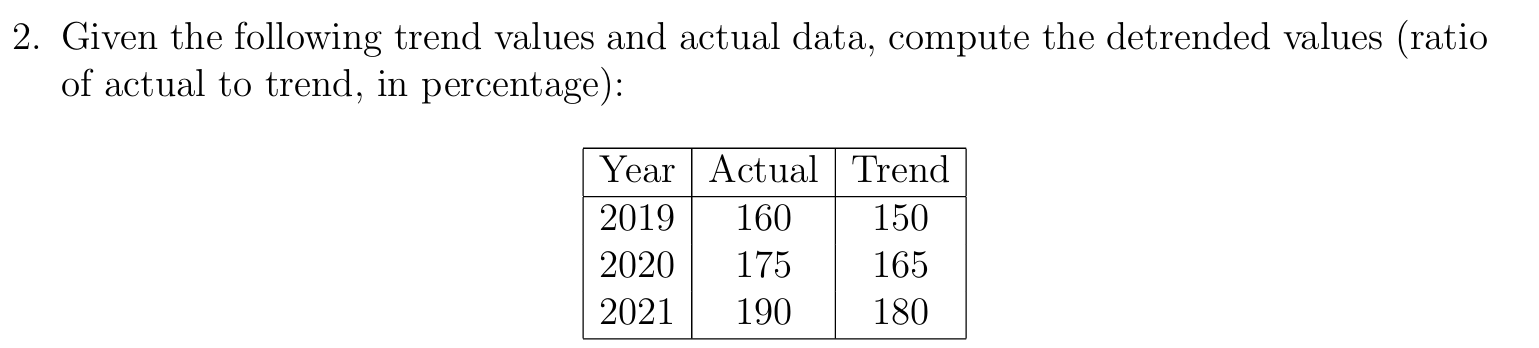
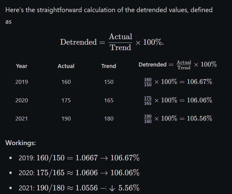
2. What is detrending? How is it carried out after fitting a trend to a time series?

Detrending is the process of removing the trend from a time series to focus on other components like seasonal or irregular variations. It helps in analyzing the fluctuations around the long-term trend.

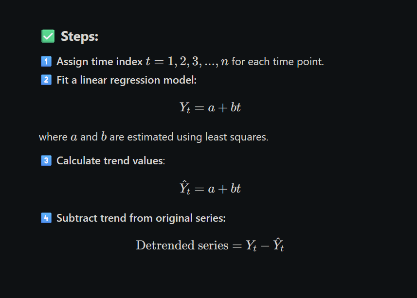
After fitting a trend to the data (using methods like moving averages or least squares), detrending is done by comparing the actual values to the trend values in two ways:

1. By Subtraction (Additive Model):

   • Detrended Value = Actual Value − Trend Value
   • Used when variations are constant over time.

2. By Division (Multiplicative Model):

   • Detrended Value = (Actual Value ÷ Trend Value) × 100
   • Gives detrended values in percentage form.
   • Used when variations change with the level of the series.

Example (Multiplicative):

If Actual Value = 150 and Trend Value = 120
→ Detrended Value = (150 ÷ 120) × 100 = 125%
→ This means the actual value is 25% above the trend.

✅ Why is it Important?

1. 📉 Makes the series stationary (constant mean), which is required for many models like ARIMA.

2. 🔍 Helps to focus on seasonal or irregular components without the influence of trend.

3. 📊 Improves the accuracy of forecasting models.

4. 🧠 Makes interpretation easier by separating the long-term movement from short-term patterns.

Steps to Detrend Using Linear Regression:

Let the time series be:

✅ Steps:

Let me know if you want help with a numerical example!

3. Discuss the effect of eliminating the trend on other components of a time series.

When we eliminate the trend from a time series (called detrending), it removes the long-term growth or decline in the data. This makes it easier to study the other components of the time series more clearly.

Effects on Other Components:

3. Seasonal Component:

   • Becomes easier to identify after removing the trend.

   • Example: Seasonal sales patterns like higher sales in festivals stand out clearly after detrending.

4. Cyclical Component:

   • Cycles in business or economy can be studied better because the general upward or downward movement (trend) is removed.

   • Example: Economic boom and recession phases can be seen more clearly.

5. Irregular/Random Component:

   • Sudden, unexpected variations (like natural disasters, strikes, etc.) are more visible after detrending.

   • These are random and don’t follow any pattern.

By removing the trend, seasonal, cyclical, and irregular variations can be analyzed more accurately. It helps in better forecasting and decision-making.

4. Describe the method of simple averages for estimating seasonal components. In what cases is it appropriate?

Definition:
The Simple Averages Method is used to measure seasonal variations in time series data. It works by calculating the average value for each season or period (like months, quarters) over several years to find the seasonal effect.

✅ Steps to Calculate:

6. Arrange Data:

   • Organize data by seasons (e.g., January sales for each year, February sales for each year, etc.).

7. Calculate Averages:

   • Find the average for each season or period.

8. Find Seasonal Indices:

   • For the multiplicative model →
     Seasonal Index = (Seasonal Average ÷ Overall Average) × 100
   • For the additive model →
     Seasonal Component = Seasonal Average − Overall Average

9. Interpret the Result:

   • These indices or values show how much a particular period differs from the overall average.

✅ When is it Appropriate?

• When data has clear and regular seasonal patterns (e.g., monthly sales, quarterly production).

• Suitable for short-term forecasting where the seasonal variation is stable over time.

✅ Example:

If the average monthly sales of a company is ₹10,000, and the average sales in December is ₹12,000 →
Seasonal Index = (12,000 ÷ 10,000) × 100 = 120%
→ This means December sales are 20% higher than the average.

✅ Conclusion:

The simple averages method is easy to use and works well for stable, regular seasonal variations in time series data.

5. What is the ratio to trend method? How is it used to estimate seasonal indices?:

Definition:
The Ratio to Trend Method is used to find seasonal indices by removing the trend from the data first and then calculating the seasonal effect.

✅ How It Is Used:

10. Find Trend Values:

    • Estimate the trend using methods like moving averages or least squares.

11. Calculate Ratios:

    • Ratio = (Actual Value ÷ Trend Value) × 100

    • This shows how much the actual value differs from the trend for each season or period.

12. Find Average Ratios:

    • For each season (e.g., January, February...), take the average of all ratios over the years.

13. Get Seasonal Indices:

    • The average ratios are used as seasonal indices to show the seasonal impact.

✅ Example:

If the Actual Sales = ₹120 and Trend Value = ₹100 →
Ratio = (120 ÷ 100) × 100 = 120%
→ Shows that sales are 20% above the trend for that month or season.

✅ When to Use:

• Useful when both trend and seasonal effects are present in the data.

• Helps to separate seasonal patterns from overall growth or decline.

✅ Conclusion:

Ratio to Trend Method helps in finding seasonal variations after removing the trend, making the data more useful for forecasting.

6. Explain the ratio to moving average method for estimating the seasonal component. What is its main advantage?

✅ Definition:

The Ratio to Moving Average Method is used to identify seasonal components in time series data.
It works by removing the trend using moving averages and then calculating seasonal effects as percentages.

✅ Steps to Apply:

14. Calculate Moving Averages:

    • Find centered moving averages of the data to estimate the trend.

15. Find Ratios:

    • Ratio = (Actual Value ÷ Moving Average) × 100
    • These ratios show how much the actual data differs from the trend for each period (month, quarter, etc.).

16. Arrange Ratios by Season:

    • Group the ratios by period (e.g., all January values, all February values, etc.).

17. Calculate Seasonal Indices:

    • Find the average of the ratios for each season.

    • These averages give the seasonal indices.

✅ Example:

Suppose Actual Sales = ₹150 and Moving Average (Trend) = ₹120
→ Ratio = (150 ÷ 120) × 100 = 125%
→ Means that sales are 25% above the trend for that month or period.

✅ Main Advantage:

• Removes both trend and cyclical variations, giving more accurate seasonal indices.

• Works well even if the trend is changing over time.

✅ Conclusion:

The Ratio to Moving Average Method gives reliable seasonal components by first removing the trend, making it very helpful in forecasting and planning.

Let me know if you want a full numerical example to practice!

7. Describe the link relatives method for computing seasonal indices. How are chain relatives formed in this method?

✅ Definition:

The Link Relatives Method is used to calculate seasonal indices by finding how each period’s value changes compared to the previous period. These changes are called link relatives.

✅ Steps to Calculate:

18. Find Link Relatives:

• Link Relative = (Current Period Value ÷ Previous Period Value) × 100
• Shows the percentage change from one period to the next.

19. Form Chain Relatives:

• Start with 100 as the first value.
• Multiply each link relative by the previous chain relative, then divide by 100 to get the next chain relative.
• Example: Next Chain Relative = (Previous Chain Relative × Link Relative) ÷ 100

20. Adjust the Chain Relatives:

• Adjust values if necessary to make the seasonal cycle consistent.

21. Calculate Seasonal Indices:

• Average the chain relatives for each season or period to find the seasonal indices.

✅ Example:

If sales in January = ₹200 and February = ₹240 →
Link Relative = (240 ÷ 200) × 100 = 120% → Sales increased by 20%.

✅ Advantages:

• Useful when data shows gradual changes over time.
• Simple to calculate seasonal indices when periods are related.

✅ Conclusion:

The Link Relatives Method helps to find seasonal patterns by studying how each period relates to the previous one, making it helpful in forecasting future trends.

Let me know if you want a numerical example to practice!

8. Compare the ratio to trend method and the ratio to moving average method for estimating seasonal components.

Here’s a simple and proper comparison in tabular form for your exam:

✅ Conclusion:
Ratio to Moving Average Method is preferred when accuracy is important, especially if the data has changing trends.
Ratio to Trend Method is useful for simpler, stable data.

Let me know if you want a numerical example of either method!

Numericals (Unit 2)

1.

1. List the data

2. Write the formula

3. Compute each 3‑year average

4. Summarize in a table

Trend Analysis

Average annual increase = (190.00 - 135.00) ÷ 4 = 13.75

Final Answer:

3-Year Moving Average Trend Values:

• 2017: 135.00
• 2018: 148.33
• 2019: 161.67
• 2020: 175.00
• 2021: 190.00

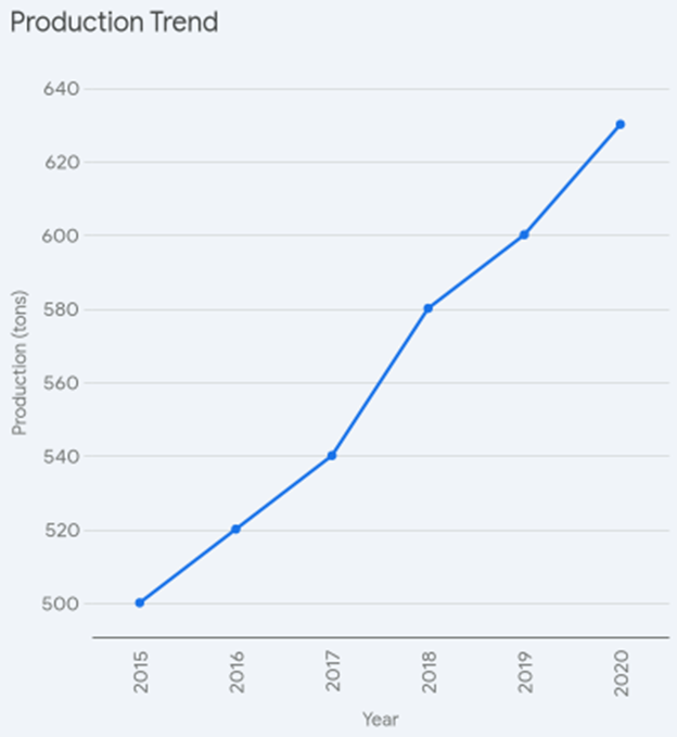
The trend shows a consistent upward pattern with an average annual increase of 13.75 units.

2.

3.

Below is a clear, step‑by‑step 4‑year moving‑average calculation:

1. Original data

2. Formula

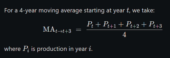
For a 4‑year moving average starting at year tt, we take:

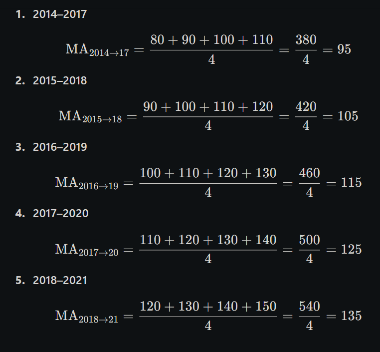
3. Compute each 4‑year average

4. Summary table

5. Notes

• You get one averaged value for each block of four consecutive years.

• Since there’s no 2013 or 2022 data, we can only form these five windows.

• These smoothed values reveal the underlying production trend without year‑to‑year “noise.”

4.

Here’s a clear, step‑by‑step calculation of the seasonal indices by the simple‑averages method:

1. Write down the data

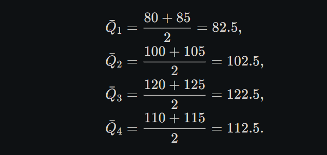
2. Compute the average for each quarter

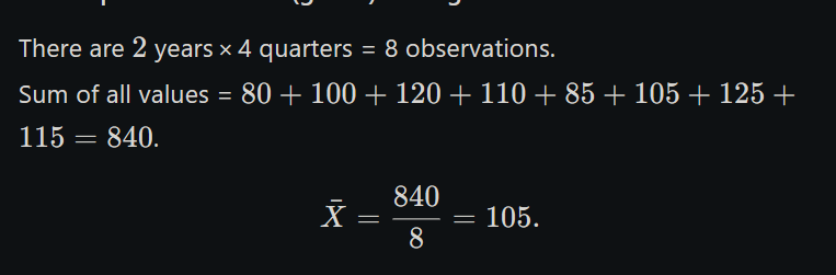
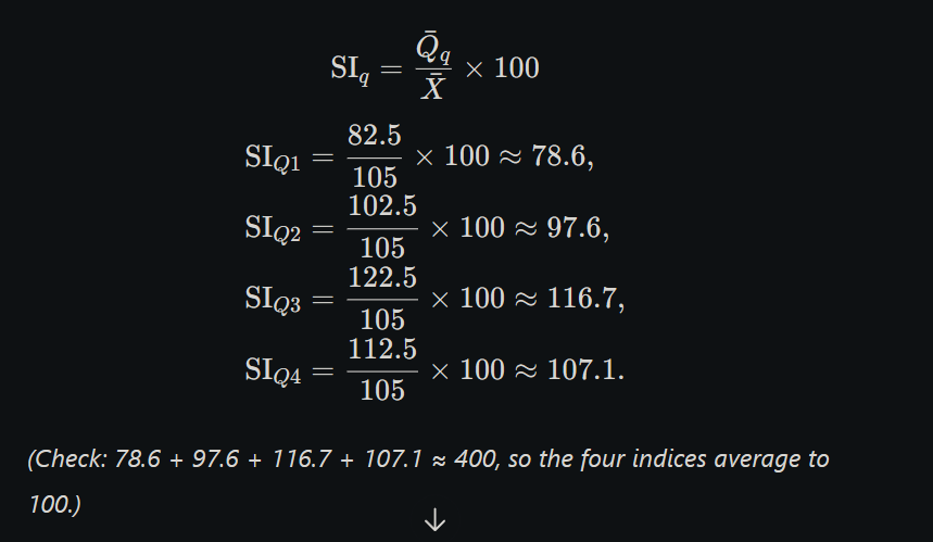
3. Compute the overall (grand) average

4. Calculate the seasonal index for each quarter

5. Present the results

Interpretation:

• A seasonal index below 100 means that in that quarter production is below the average—Q1 is the weakest (78.6).

• An index above 100 means that quarter is stronger than average—Q3 is the strongest (116.7).

This completes the simple‑averages seasonal‑index calculation.

5.

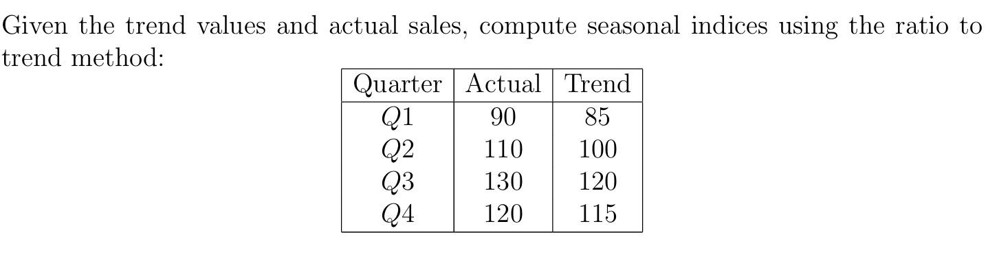
Below is a clear, step‑by‑step “ratio‐to‐trend” calculation of the seasonal indices. We’ll first compute the raw ratios (Actual / Trend × 100), then normalize them so that their sum = 4 × 100 = 400.

1. Tabulate the data

2. Compute raw seasonal ratios

Raw Indexq=ActualqTrendq×100\text{Raw Index}_q = \frac{\text{Actual}_q}{\text{Trend}_q}\times 100

Sum of raw indices = 90.00 + 91.67 + 108.33 + 73.91 = 363.91

3. Compute normalization factor

We want the four normalized indices to average 100 (i.e. sum to 400).

4. Compute final (normalized) seasonal indices

(Check: 98.9 + 100.7 + 119.1 + 81.3 ≈ 400)

5. Interpretation

• Q3 has the strongest seasonality (≈ 119), meaning sales tend to be about 19 % above trend in that quarter.

• Q4 is the weakest (≈ 81), about 19 % below trend.

• Q1 and Q2 are fairly close to trend (≈ 99 and 101).

This completes the 5‑mark ratio‑to‑trend method.

Unit 3

1. Define forecasting. What are the main goals and applications of forecasting in business and economics?

22. Definition
    Forecasting is the process of predicting future events or values by analyzing historical data, current trends, and relevant qualitative factors.

23. Main Goals

    • Planning & Resource Allocation: Anticipate demand to size production, inventory, staffing, and budgets.

    • Risk Management: Spot potential challenges or opportunities and prepare contingency plans.

    • Decision Support: Provide quantitative inputs for strategic choices (e.g., investment, pricing).

24. Key Business Applications

    • Sales & Marketing: Demand forecasts, market‐share estimates, pricing strategies.

    • Operations: Production scheduling, supply‑chain optimization, maintenance planning.

    • Finance: Cash‑flow projections, budget setting, capital‑allocation decisions.

25. Key Economic Applications

    • Macroeconomic Planning: GDP, inflation, employment, interest‑rate projections.

    • Sectoral Analysis: Industry growth trends, commodity‐price forecasts, trade‐balance estimates.

    • Policy Formulation: Inputs for fiscal (tax/spend) and monetary (rate) decisions.

26. Benefits

    • Reduces uncertainty and supports evidence‑based planning

    • Improves efficiency and cost control

    • Enhances competitive advantage and strategic agility

2. Differentiate between qualitative and quantitative forecasting methods. Give two examples of each.

Below is a consolidated comparison in a single, clear table format:

3. Variate Component Method in Time Series Analysis

Definition:
The variate component method is a technique used to break a time series into four key components to better understand its behavior and to improve forecasting. It assumes that a time series is formed by systematic patterns along with random variations.

Mathematical Form:

• Additive: Yt = Tt + St + Ct + It

• Multiplicative: Yt = Tt × St × Ct × It
  Where:
  Yt = Observed value at time t

Key Components:

27. Trend (Tt):

• Definition: The long-term movement in data.

• Shows: General increase, decrease, or stability over time.

• Example: Growth of population or company sales over years.

28. Seasonal (St):

• Definition: Regular, repeating patterns at fixed intervals (like months or quarters).

• Cause: Weather, festivals, or business cycles.

• Example: Higher ice cream sales in summer, peak retail sales in December.

29. Cyclical (Ct):

• Definition: Long-term up and down movements without fixed periods, linked to business cycles.

• Example: Stock market booms and recessions, housing market cycles.

30. Irregular (It):

• Definition: Random fluctuations that cannot be explained by other components.

• Cause: Natural disasters, sudden economic changes, errors.

• Example: Sales drop due to a sudden flood or a strike.

Process of Decomposition:

31. Identify and remove the trend.

32. Analyze and extract the seasonal component.

33. Examine for cyclical patterns.

34. The leftover is the irregular component.

Importance:

• Helps in accurate forecasting.

• Useful in business planning.

• Helps identify seasonal trends and unusual events.

Example:

• Electricity Consumption:
  → Increasing trend (more appliances used),
  → Higher usage in summers (seasonal),
  → Fluctuations due to economy (cyclical),
  → Sudden spike due to heatwave (irregular).

Conclusion:
The variate component method simplifies complex time series by breaking it into trend, seasonal, cyclical, and irregular parts, making analysis and forecasting more effective.

4. When would you choose an additive model over a multiplicative model in time series decomposition? Explain with examples.

Additive Model:
Yt = Tt + St + It
(Where Yt = observed data, Tt = trend, St = seasonal component, It = irregular component)

Multiplicative Model:
Yt = Tt × St × It

When to Use Additive Model:

• Choose additive model when seasonal variations remain constant in absolute terms over time.

• It is used when seasonal effects do not depend on the trend or data level.

• Seasonal fluctuations add a fixed amount to the trend.

Example (Additive Model):
Monthly temperature:

• Year 1: Jan = 5°C, Jul = 25°C → Difference = 20°C

• Year 10: Jan = 7°C, Jul = 27°C → Difference = 20°C
  → Same difference = Additive model suitable.

When to Use Multiplicative Model:

• Choose multiplicative model when seasonal variations increase or decrease proportionally with the trend.

• Used when percentage seasonal variation stays constant over time.

Example (Multiplicative Model):
Monthly sales:

• Year 1: Jan = 1000 units, Dec = 1500 units → 50% increase

• Year 10: Jan = 4000 units, Dec = 6000 units → 50% increase
  → Constant percentage = Multiplicative model suitable.

Summary Table:

Conclusion:

Use additive model when seasonal effects are fixed amounts, and multiplicative model when seasonal effects are proportional to the trend. Choosing the correct model improves forecasting accuracy.

5. What is a stationary time series? Distinguish between strict stationarity and weak stationarity.

Stationary Time Series (Definition):
A time series is said to be stationary if its statistical properties like mean, variance, and autocovariance remain constant over time. It shows no long-term trends, seasonal patterns, or systematic changes. Stationarity is important in time series analysis because many forecasting methods require it.

Types of Stationarity:

35. Strict Stationarity:
    A time series is strictly stationary if the entire probability distribution of the series remains unchanged over time. This means that not just the mean and variance, but all moments (mean, variance, skewness, kurtosis, etc.) are constant.

• Example: White noise process.
• Note: Very strict and rarely found in real-world data.

36. Weak Stationarity (Covariance Stationarity):
    A time series is weakly stationary if only its mean, variance, and autocovariance are constant over time, and autocovariance depends only on the gap (lag) between observations.

• Example: Many financial return series.
• Note: Most practical and widely used form of stationarity.

Differences Between Strict and Weak Stationarity:

Relation:

Strict stationarity → Weak stationarity (if variance exists)
Weak stationarity ↛ Strict stationarity

6. Define autocorrelation function (ACF). How does it help in identifying the structure of a time series?

5‑Mark Answer on the Autocorrelation Function (ACF)

37. Definition (1 mark)
    The ACF at lag h is the correlation between a time‐series and itself shifted by h periods. Formally:

    ρ(h)=Cov(Yt, Yt−h)Var(Yt). \rho(h) = \frac{\mathrm{Cov}(Y_t,,Y_{t-h})}{\mathrm{Var}(Y_t)}.

38. Key Pattern Signatures (1 mark)

    • White Noise: ρ(0)=1; ρ(h)=0 for h≠0

    • AR(1): ρ(h)=φʰ (exponential decay)

    • Seasonal: Peaks at seasonal lags (e.g., h=12,24,… for monthly)

39. Stationarity & Trend Detection (1 mark)

    • Stationary: ACF drops to (near) zero quickly

    • Non‑stationary/Trend: ACF decays slowly, remaining high over many lags

40. Model Identification (1 mark)

    • AR(p): Gradual/exponential decay (no abrupt cut‑off)

    • MA(q): Cut‑off after lag q (ρ(h)=0 for h>q)

    • ARMA(p,q): Combination—neither pure cut‑off nor simple decay

41. Applications (1 mark)

    • Selecting ARIMA(p,d,q): Identify p (decay pattern) and q (cut‑off)

    • Seasonal Modeling: Detect seasonal lags

    • Stationarity Testing: Decide on differencing (if ACF decays slowly)

Each of these points addresses a core use of the ACF, totaling five succinct marks.

7. What is a correlogram? How is it useful in time series analysis?

5‑Mark Answer on Correlograms

42. Definition (1 mark)
    A correlogram is a bar chart of autocorrelation coefficients ρ(h) plotted against lags h, showing how a time series correlates with its past values.

43. Key Components (1 mark)

    • X‑axis: Lag h (e.g. 0, 1, 2, …)

    • Y‑axis: Autocorrelation ρ(h) (range –1 to +1)

    • Bars: Height = ρ(h) at each lag

    • Confidence Bounds: Dashed lines at ±1.96/√n to flag statistically significant lags

44. Pattern Recognition (1 mark)

    • Trend (Non‑stationary): Correlogram decays slowly (high ρ for many lags)

    • Stationary: Rapid drop to near zero

    • Seasonality: Repeating peaks at seasonal lags (e.g. h=12, 24 for monthly data)

45. Model Identification (1 mark)

    • AR(p): Exponential/damped decay in ρ(h)

    • MA(q): Sharp cutoff after lag q (ρ(h)=0 for h>q)

    • ARMA(p,q): Mixed pattern—neither pure cutoff nor simple decay

46. Practical Use (1 mark)

    • Stationarity Check: Decide if differencing is needed

    • ARIMA Setup: Choose p (decay) and q (cutoff)

    • Seasonal Modeling: Identify seasonal periods for inclusion in the model

Three-Month Moving Average and Seasonal Analysis

Given Data - Monthly Sales Revenue (20X2)

Step 1: Calculate Three-Month Moving Averages

Formula: 3-Month MA = (Month₁ + Month₂ + Month₃) ÷ 3

Detailed Calculation Table

Step 2: Results Summary Table

Sales vs. Moving Average Comparison

Step 3: Seasonal Variation Analysis

Pattern Identification Table

Seasonal Indices Calculation

Base: Moving Average as 100

Step 4: Seasonal Pattern Analysis

Clear Seasonal Cycle Identified:

Quarterly Pattern:

Monthly Seasonal Categories:

47. Peak Months (Mar, Jun, Sep, Dec): Index ~120

    • Sales 20% above trend
    • Likely due to seasonal demand/holidays

48. Low Months (Apr, Jul, Oct): Index ~84-85

    • Sales 15-16% below trend
    • Post-peak adjustment periods

49. Moderate Months (Feb, May, Aug, Nov): Index ~95-96

    • Sales 4-5% below trend
    • Transition/building periods

Step 5: Key Findings

Trend Analysis:

• Overall Trend: Gradually increasing from 152.0 to 170.0
• Monthly Growth: Average increase of 1.8 per month
• Annual Growth Rate: Approximately 11.8%

Seasonal Variation:

• High Variability: Range from 84.0 to 120.8 (36.8 point spread)
• Predictable Pattern: 3-month cycle repeating quarterly
• Seasonality Strength: ±20% deviation from trend

Business Implications:

50. Inventory Planning: Stock up before Mar, Jun, Sep, Dec
51. Cash Flow: Expect higher revenues in peak months
52. Staffing: Plan for increased activity in peak periods
53. Marketing: Focus campaigns before peak months

Final Summary:

Three-Month Moving Averages:

Seasonal Pattern:

• Clear 3-month cycle: Peak → Moderate → Low
• Peak months: Mar, Jun, Sep, Dec (120% of trend)
• Low months: Apr, Jul, Oct (84% of trend)
• Moderate months: Feb, May, Aug, Nov (96% of trend)